Show code cell content
import numpy as np
import matplotlib.pyplot as plt
plt.style.use("https://github.com/mlefkir/beauxgraphs/raw/main/beautifulgraphs_colblind.mplstyle")
On the Fast Fourier Transform to compute the autocovariance#
Here we show the effects of computing the autocovariance function (ACVF) using the Fast Fourier Transform. We will show these effects using functions where we know the analytical Fourier Transform. Which are the exponential and squared exponential autocovariance functions. First we compute the ACVF on an arbitrary grid and then we compute the ACVF on an extended grid of frequencies.
Autocovariance \(R(\tau)\) |
Power spectrum \(\mathcal{P}(f)\) |
|
|---|---|---|
Exponential |
\(\dfrac{A}{2\gamma} \exp{(-|\tau|\gamma)}\) |
\(\dfrac{A}{\gamma^2 +4\pi^2 f^2}\) |
Squared exponential |
\(A\exp{(-2 \pi^2 \tau^2 \sigma^2)}\) |
\(\dfrac{A}{\sqrt{2\pi}\sigma}\) \(\exp\left(-\dfrac{f^2}{2\sigma^2} \right)\) |
Arbitrary grid of frequencies#
Squared exponential ACVF#
First, we define the autocovariance function and its Fourier transform, i.e. the power spectrum.
Show code cell content
def SqExpo_ACV(t, A, sigma):
    return A * np.exp( -2 * np.pi**2 * sigma**2 * t**2 )

def SqExpo_PSD(f, A, sigma):
    return A / (np.sqrt(2*np.pi) * sigma ) * np.exp( - 0.5 * f**2 / sigma**2 )
We generate a grid of frequencies from \(0\) to \(f_N\) with a spacing \(\Delta f=f_0\). The power spectrum will be of length \(N\).
f0 = 1e-4 # min frequency
df = f0
fN = 5. # max frequency
# grid of frequencies, from 0 to fend-df with step size df
f = np.arange(0,fN,df)
# number of points in the psd including the zeroth freq
N = len(f)
# define the parameters of the psd
A , sigma = 1 , 1.e-1

P = SqExpo_PSD(f,A,sigma)
Show code cell source
fig,ax = plt.subplots(1,1,figsize=(7,4.5))
ax.plot(f,P,'.')
ax.set_xlabel(r'$f$')
ax.set_ylabel('Power spectral density')
ax.loglog()
ax.set_title("Squared exponential")
fig.tight_layout()

As we know the power spectrum is symmetric for negative frequencies, we can use the real inverse Fourier transform to compute the autocovariance function.
We use the function np.fft.irfft to compute the inverse Fourier transform. The discrete inverse Fourier transform returns a real array of length \(2N-2\). Where x[0] is the autocovariance at \(\tau=0\) and x[N-1] is the autocovariance at \(\tau=\tau_\mathrm{max}\), after which the autocovariance is mirrored for negative lags. The time separation between the autocovariance values is given by \(\Delta \tau = \tau_\mathrm{max}/(N-1)\), where \(\tau_\mathrm{max}=1/2\Delta f\) is the maximum lag for which we compute the autocovariance function.
To obtain the true autocovariance function we divide the result by the sampling frequency \(\Delta f\).
tmax = 0.5 / df
dt = 1/df/(N-1)/2

t = np.arange(0,tmax+dt,dt)

R_theo = SqExpo_ACV(t,A,sigma) # theoretical inverse FT of the lorentzian

# compute the IFFT, with a normalisation factor 1/M, M=2*(len(y)-1)
R_dift = np.fft.irfft(P)
assert (R_dift[1:N-1]-np.flip(R_dift[N:])<np.finfo(float).eps).all(), "The IRFFT did not return a mirrored ACV"
R_num = R_dift[:N]/dt
Below, we plot the resulting autocovariance function and the error between the numerical and analytical autocovariance function. For plotting purposes, we only plot the autocovariance function for positive lags and up to \(\tau=10\).
We can see that in the case of the squared exponential autocovariance function, the numerical Fourier transform is exact within the numerical precision.
Show code cell source
fig,ax = plt.subplots(1,2,figsize=(9,4.5))
ax[0].plot(t,R_theo,label='Analytical')#,marker='s')
ax[0].plot( t, R_num,label='Numerical',marker='o')

ax[0].legend()
ax[0].set_xlim(-1e-5,10 )
ax[0].set_xlabel(r"$\tau$")
ax[0].set_ylabel(r"Autocovariance function")
ax[1].plot(t,np.abs(R_theo-R_num),label='|Error|')#,marker='s')

ax[1].set_xlabel(r"$\tau$")
ax[1].set_ylabel(r"Absolute difference")
fig.suptitle("Inverse Fourier transform of the Squared exponential PSD")
fig.tight_layout()

We can check the Fourier pairs properties of the autocovariance function and the power spectrum by comparing the sums.
Show code cell source
print(f"P(0)           : {P[0]:1.5e}")
print(f'Sum of ACV     : {np.trapz(R_num)*dt*2:1.5e}')
print(f'Sum of ACVtheo : {np.trapz(R_theo)*dt*2:1.5e}')
print(f"------Error----: {np.abs(np.trapz(R_num)*2*dt-P[0]):1.5e}\n")

print(f'Sum of PSD     : {np.trapz(P)*df*2:1.3e}')
print(f'ACVtheo[0]     : {(R_theo[0]):1.3e}')
print(f'ACV[0]         : {R_num[0]:1.3e}')
print(f"-----Error-----: {np.abs(np.trapz(P)*2*df-R_num[0]):1.3e}\n")
P(0)           : 3.98942e+00
Sum of ACV     : 3.98942e+00
Sum of ACVtheo : 3.98942e+00
------Error----: 1.33227e-15

Sum of PSD     : 1.000e+00
ACVtheo[0]     : 1.000e+00
ACV[0]         : 1.000e+00
-----Error-----: 0.000e+00
Exponential ACVF#
Show code cell content
def Expo_PSD(f, A, gamma):
    return A / ( (4*np.pi**2 * f**2 + gamma**2) )
def Expo_ACV(t, A, gamma):
    return 0.5* A / gamma * np.exp( - gamma * t )
f0 = 1e-3
df = f0
fN = 1. # max frequency
f = np.arange(0,fN,df)
N = len(f)
A , sigma = 1 , 1e-1
P = Expo_PSD(f,A,sigma)
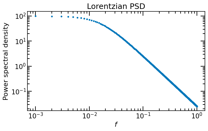
Unlike in the previous case, the power spectrum is less steep, it does not decay as fast to zero. This means that the autocovariance function at the firs time lags will be more affected by the numerical Fourier transform.
Show code cell source
fig,ax = plt.subplots(1,1,figsize=(7,4.5))
ax.plot(f,P,'.')
ax.set_xlabel(r'$f$')
ax.set_ylabel('Power spectral density')
ax.loglog()
ax.set_title("Lorentzian PSD")
fig.tight_layout()
Show code cell source
tmax = 0.5 / df
dt = 1/df/(N-1)/2

t = np.arange(0,tmax+dt,dt)

R_theo = Expo_ACV(t,A,sigma)

# compute the IFFT, with a normalisation factor 1/M, M=2*(len(y)-1)
R_dift = np.fft.irfft(P)
# assert (R_dift[1:N-1]-np.flip(R_dift[N:])<np.finfo(float).eps).all(), "The IRFFT did not return a mirrored ACV"
R_num = R_dift[:N]/dt
We see that this time FFT does not give an exact result within the numerical precision, this is due to the power spectrum does not decay as fast to zero as in the case of the squared exponential autocovariance function. The Discrete Fourier Transform assumes the signal is periodic, the power spectrum is replicated at the end of the grid of frequencies but because the power spectrum does not decay to zero, the aliasing effect is more important. We will see how to mitigate this effect in the next section.
Show code cell source
fig,ax = plt.subplots(1,2,figsize=(9,4.5))
ax[0].plot(t,R_theo,label='Analytical')
ax[0].plot( t, R_num,label='Numerical',marker='o')

ax[0].legend()
ax[0].set_xlim(-1e-5,60 )
ax[0].set_xlabel(r"$\tau$")
ax[0].set_ylabel(r"Autocovariance function")
ax[1].plot(t,np.abs(R_theo-R_num),label='|Error|')#,marker='s')

ax[1].set_xlabel(r"$\tau$")
ax[1].set_ylabel("Absolute difference")
ax[1].set_xlim(-1e-5,20 )

fig.suptitle("Inverse Fourier transform of the Lorentzian PSD")
fig.tight_layout()

Show code cell source
print(f"P(0)           : {P[0]:1.5e}")
print(f'Sum of ACV     : {np.trapz(R_num)*dt*2:1.5e}')
print(f'Sum of ACVtheo : {np.trapz(R_theo)*dt*2:1.5e}')
print(f"------Error----: {np.abs(np.trapz(R_num)*2*dt-P[0]):1.5e}\n")

print(f'Sum of PSD     : {np.trapz(P)*df*2:1.3e}')
print(f'ACVtheo[0]     : {(R_theo[0]):1.3e}')
print(f'ACV[0]         : {R_num[0]:1.3e}')
print(f"-----Error-----: {np.abs(np.trapz(P)*2*df-R_num[0]):1.3e}\n")
P(0)           : 1.00000e+02
Sum of ACV     : 1.00000e+02
Sum of ACVtheo : 1.00021e+02
------Error----: 2.84217e-14

Sum of PSD     : 4.949e+00
ACVtheo[0]     : 5.000e+00
ACV[0]         : 4.949e+00
-----Error-----: 0.000e+00
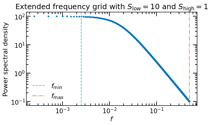
Extending the grid of frequencies#
As we saw in the previous section, the autocovariance obtained via FFT on a grid of frequencies can be affected by the aliasing effect. To mitigate this effect, we can extend the grid of frequencies.
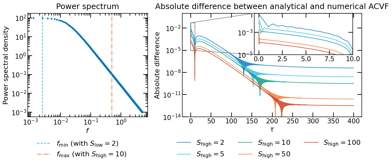
Let us consider the case of a signal of duration \(T=400\) with a sampling period of \(\Delta T=1\). We want to compute the ACVF of the signal given our two PSD models. The minimal grid of frequencies to compute the ACVF is \(f_\mathrm{min}=1/T\) and the maximal grid of frequencies is given by the Nyquist frequency \(f_\mathrm{max}=1/2\Delta T\). As we saw in the previous section, the autocovariance obtained via FFT on a grid of frequencies can be affected by aliasing.
To mitigate this effect, we extend the grid of frequencies with two factors: \(S_\mathrm{low}\) and \(S_\mathrm{high}\), for low and high frequencies, respectively. The grid of frequencies is then given by \(f_0 = f_\mathrm{min}/S_\mathrm{low} = \Delta f\) to \(f_N = f_\mathrm{max}S_\mathrm{high}=N \Delta f\).