Show code cell content
import jax.numpy as jnp
import matplotlib.pyplot as plt
plt.style.use("https://github.com/mlefkir/beauxgraphs/raw/main/beautifulgraphs_colblind.mplstyle")
Modelling with an autocovariance function#
The autocovariance function of the time series is represented by the object CovarianceFunction. More details about this class and the implemented models can be found in acvf. We will describe how to use, combine and create models for the autocovariance function in the following sections.
A first model#
We show how to use the models implemented in acvf to compute the autocovariance at given time lags. We first define an instance of the chosen class. In this example, we create instances of the classes Exponentialand Matern32.
The values of the parameters of the models are given as a list of floats, during instantiation.
from pioran.acvf import Exponential, Matern32

Expo = Exponential([1, 0.5])
Mat32 = Matern32([1.2, 0.5])
A CovarianceFunction object has a field parameters which an object of the class ParametersModel storing for the parameters of the model. We can inspect the values of the parameters of the model by printing the CovarianceFunction object.
print(Mat32)
Covariance function: matern32
Number of parameters: 2
============================================================================
CID  ID   Name            Value          Status    Linked    Type
1    1    variance        1.2            Free      No        Hyper-parameter
1    2    length          0.5            Free      No        Hyper-parameter

Number of free parameters : 2
If we want to change the values of the parameters of the model, we can use the method set_free_values on the attributeCovarianceFunction.parameters. The method takes as input a list of floats, which are the values of the free parameters of the model. Currently, it is not possible to change the values of the fixed parameters of the model after instantiation. To do so, we need to create a new instance of the model and set the parameters as free or fixed using the keyword argument free_parameters. More details about the class ParametersModel can be found parameters.
Mat32.parameters.set_free_values([2.2, 1.5])
print(Mat32)
Covariance function: matern32
Number of parameters: 2
============================================================================
CID  ID   Name            Value          Status    Linked    Type
1    1    variance        2.2            Free      No        Hyper-parameter
1    2    length          1.5            Free      No        Hyper-parameter

Number of free parameters : 2
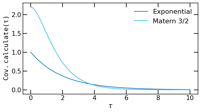
We can evaluate the autocovariance function at given time lags by calling the method calculate of the CovarianceFunction object. The method calculate takes as input a list of floats representing the time lags at which the autocovariance function is evaluated. The method returns a list of floats representing the values of the autocovariance function at the given time lags.
Show code cell source
t = jnp.linspace(0, 10, 1000)

fig, ax = plt.subplots(1, 1, figsize=(7, 4))
ax.plot(t, Expo.calculate(t), label="Exponential")
ax.plot(t, Mat32.calculate(t), label="Matern 3/2")
ax.set_xlabel(r'$\tau$')
ax.set_ylabel(r'$\tt{Cov.calculate}(\tau)$')
ax.legend()
fig.tight_layout()
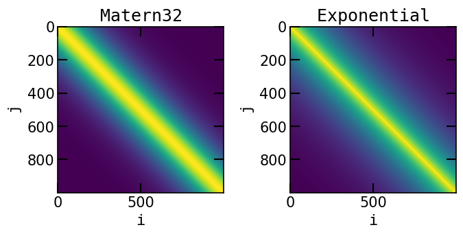
The covariance matrix can be obtained by calling the method get_cov_matrix(). This method takes in input two arrays of shape \((N,1)\) and \((M,1)\) representing the time lags at which the covariance matrix is evaluated. The method returns a matrix of shape \((N,M)\) representing the covariance matrix at the given time lags.
K_Mat32 = Mat32.get_cov_matrix(t.reshape(-1, 1), t.reshape(-1, 1))
K_expo = Expo.get_cov_matrix(t.reshape(-1, 1), t.reshape(-1, 1))
Show code cell source
fig, ax = plt.subplots(1, 2, figsize=(7, 4))

ax[0].imshow(K_Mat32)
ax[0].set_xlabel(r'$\tt{i}$')
ax[0].set_ylabel(r'$\tt{j}$')
ax[0].set_title(r'$\tt{Matern32}$')

ax[1].imshow(K_expo)
ax[1].set_xlabel(r'$\tt{i}$')
ax[1].set_ylabel(r'$\tt{j}$')
ax[1].set_title(r'$\tt{Exponential}$')
fig.tight_layout()
Combining autocovariance functions#
In this section, we show how to combine autocovariance functions via arithmetic operations.
In this example we create instances of the classes Exponential, SquaredExponential and Matern32.
from pioran.acvf import Exponential, Matern32, SquaredExponential

Expo = Exponential([1.68, 0.75])
Mat32 = Matern32([.33, 1.5])
SqExpo = SquaredExponential([1.45, 0.5])
Sum of autocovariance functions#
We can create a model which is the sum of the three components by using the + operator. The result is a new instance of the class CovarianceFunction. We can inspect the parameters of the model by printing the object.
Model = Expo + Mat32 + SqExpo
print(Model)
Covariance function: exponential + matern32 + squared_exponential
Number of parameters: 6
============================================================================
CID  ID   Name            Value          Status    Linked    Type
1    1    variance        1.68           Free      No        Hyper-parameter
1    2    length          0.75           Free      No        Hyper-parameter
2    3    variance        0.33           Free      No        Hyper-parameter
2    4    length          1.5            Free      No        Hyper-parameter
3    5    variance        1.45           Free      No        Hyper-parameter
3    6    length          0.5            Free      No        Hyper-parameter

Number of free parameters : 6
Because several parameters have identical names it is necessary to use the indices of the parameters to access them. CID gives the component index and ID gives the parameter index in the whole model.
print(Model.parameters[5])
3 5 variance 1.45 Free No Hyper-parameter
As previously, we can change the values of the free parameters:
Model.parameters.set_free_values([13.68, 0.975, 0.339, 1.95, 1.345, 3.5])
print(Model)
Covariance function: exponential + matern32 + squared_exponential
Number of parameters: 6
============================================================================
CID  ID   Name            Value          Status    Linked    Type
1    1    variance        13.68          Free      No        Hyper-parameter
1    2    length          0.975          Free      No        Hyper-parameter
2    3    variance        0.339          Free      No        Hyper-parameter
2    4    length          1.95           Free      No        Hyper-parameter
3    5    variance        1.345          Free      No        Hyper-parameter
3    6    length          3.5            Free      No        Hyper-parameter

Number of free parameters : 6
Show code cell source
t = jnp.linspace(0, 10, 1000)

fig, ax = plt.subplots(1, 1, figsize=(7, 4))

ax.plot(t, Expo.calculate(t), label="Exponential", lw=2,ls="--")
ax.plot(t, Mat32.calculate(t), label="Matern 3/2", lw=2,ls="--")
ax.plot(t, SqExpo.calculate(t), label="Squared Exponential", lw=2,ls="--")
ax.plot(t, Model.calculate(t), label="Sum of the three")
ax.set_xlabel(r'$\tau$')
ax.set_ylabel(r'$\tt{Cov.calculate}(\tau)$')
ax.legend()
fig.tight_layout()

Product of autocovariance functions#
We can create a model which is a product of covariance functions by using the * operator. The result is a new instance of the class CovarianceFunction. We show an example with the product of the two first components plus the third component.
Expo = Exponential([1.68, 0.75])
Mat32 = Matern32([.33, 1.5])
SqExpo = SquaredExponential([.45, 0.5])

Model = Expo * Mat32+ SqExpo
print(Model)
Covariance function: exponential * matern32 + squared_exponential
Number of parameters: 6
============================================================================
CID  ID   Name            Value          Status    Linked    Type
1    1    variance        1.68           Free      No        Hyper-parameter
1    2    length          0.75           Free      No        Hyper-parameter
2    3    variance        0.33           Free      No        Hyper-parameter
2    4    length          1.5            Free      No        Hyper-parameter
3    5    variance        0.45           Free      No        Hyper-parameter
3    6    length          0.5            Free      No        Hyper-parameter

Number of free parameters : 6
Show code cell source
t = jnp.linspace(0, 10, 1000)

fig, ax = plt.subplots(1, 1, figsize=(7, 4))

ax.plot(t, Expo.calculate(t), label="Exponential", lw=2,ls="--")
ax.plot(t, Mat32.calculate(t), label="Matern 3/2", lw=2,ls="--")
ax.plot(t, SqExpo.calculate(t), label="Squared Exponential", lw=2,ls="--")
ax.plot(t, Model.calculate(t), label="Expo * Matern 3/2 + Sq Expo")
ax.set_xlabel(r'$\tau$')
ax.set_ylabel(r'$\tt{Cov.calculate}(\tau)$')
ax.legend()
fig.tight_layout()

Writing a new model#
Here we show how to write a new model for the autocovariance function, which can be used like any models we have shown above.
Creating the class and the constructor#
We write a new class MyAutocovariance, which inherits from CovarianceFunction. It is important to specify the attributes parameters and expression at the class level as CovarianceFunction inherits from Module. parameters is an object of the class ParametersModel which is a container for the parameters of the model. The constructor __init__ must be defined as in the example and the names of the parameters are given in the param_names list.
The calculate method#
The calculate method must be defined and it must return the autocovariance function evaluated at the time t. When writing the expression of the autocovariance function, the values of parameters of the model can be accessed using the attribute self.parameters['name'].value where name is the name of the parameter.
This method is then called by the method get_cov_matrix() to compute for instance the likelihood or the posterior predictive distribution of a Gaussian process.
import jax.numpy as jnp
from pioran import CovarianceFunction
from pioran.parameters import ParametersModel

class MyAutocovariance(CovarianceFunction):
    parameters: ParametersModel
    expression = 'name of the model'

    def __init__(self, param_values, free_parameters=[True, True, True]):
        """Constructor of the covariance function inherited
        from the CovarianceFunction class.
        """
        assert len(param_values) == 3, 'The number of parameters must be 3'
        CovarianceFunction.__init__(self, param_values=param_values,
        param_names=['variance', 'length','period'], free_parameters=free_parameters)

    def calculate(self,t):
        """Returns the autocovariance function evaluated at t.
        """
        return  self.parameters['variance'].value *jnp.exp(- jnp.abs(t) * self.parameters['length'].value)*jnp.cos(2*jnp.pi*t / self.parameters['period'].value)
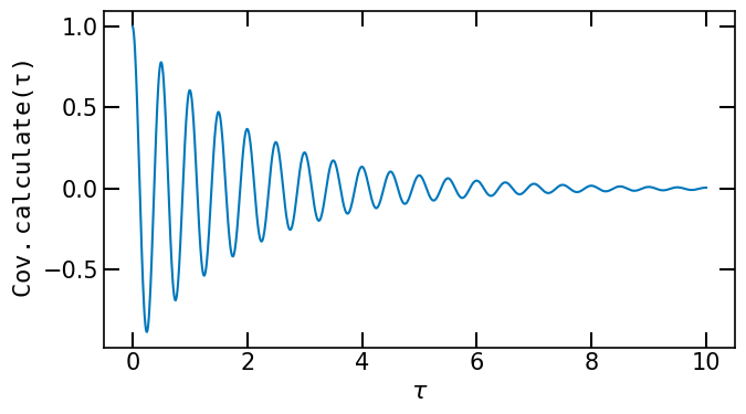
We can use the newly defined model as any other models we have shown above:
Cov = MyAutocovariance([1., 0.5,.5])
taus = jnp.linspace(0, 10, 1000)
avc = Cov.calculate(taus)
Show code cell source
fig, ax = plt.subplots(1,1,figsize=(7,4))
ax.plot(taus, avc)
ax.set_xlabel(r'$\tau$')
ax.set_ylabel(r'$\tt{Cov.calculate}(\tau)$')
fig.tight_layout()