Show code cell content Hide code cell content

import jax.numpy as jnp
import matplotlib.pyplot as plt
plt.style.use("https://github.com/mlefkir/beauxgraphs/raw/main/beautifulgraphs_colblind.mplstyle")

Modelling with a power spectral density

The power spectral density function of the time series is represented by the object PowerSpectralDensity. More details about this class and the implemented models can be found psd. We will describe how to use, combine and create models for the power spectral density function in the following sections.

A first model

We show how to use the models implemented in pioran.psd to compute the power spectrum at given frequencies. We first define an instance of the chosen class. In this example, we create instances of the classes Lorentzian and Gaussian.

The values of the parameters of the models are given as a list of floats, during instantiation.

from pioran.psd import Lorentzian, Gaussian

Lore = Lorentzian([0,1, 0.5])
Gauss = Gaussian([0,1.2, 0.5])

A PowerSpectralDensity object has a field parameters which an object of the class ParametersModel storing for the parameters of the model. We can inspect the values of the parameters of the model by printing the PowerSpectralDensity object.

print(Lore)

Power spectrum: lorentzian
Number of parameters: 3
============================================================================
CID  ID   Name            Value          Status    Linked    Type            
1    1    position        0              Free      No        Hyper-parameter 
1    2    amplitude       1              Free      No        Hyper-parameter 
1    3    halfwidth       0.5            Free      No        Hyper-parameter 

Number of free parameters : 3

If we want to change the values of the parameters of the model, we can use the method set_free_values on the attributePowerSpectralDensity.parameters. The method takes as input a list of floats, which are the values of the free parameters of the model. Currently, it is not possible to change the values of the fixed parameters of the model after instantiation. To do so, we need to create a new instance of the model and set the parameters as free or fixed using the keyword argument free_parameters. More details about the class ParametersModel can be found in the API.

Lore.parameters.set_free_values([0.9,2.2, 1.5])
print(Lore)

Power spectrum: lorentzian
Number of parameters: 3
============================================================================
CID  ID   Name            Value          Status    Linked    Type            
1    1    position        0.9            Free      No        Hyper-parameter 
1    2    amplitude       2.2            Free      No        Hyper-parameter 
1    3    halfwidth       1.5            Free      No        Hyper-parameter 

Number of free parameters : 3

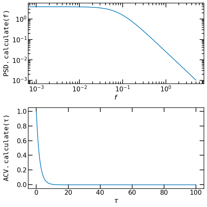
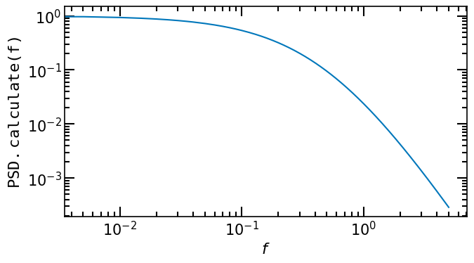
We can evaluate the PSD at given frequencies by calling the method calculate of the PowerSpectralDensity object. The method calculate takes as input a list of floats representing the frequencies at which the PSD is evaluated. The method returns a list of floats representing the values of the PSD at the given frequencies.

Show code cell source Hide code cell source

t = jnp.linspace(0, 10, 1000)

fig, ax = plt.subplots(1, 1, figsize=(7, 4))
ax.plot(t, Gauss.calculate(t), label="Gaussian")
ax.plot(t, Lore.calculate(t), label="Lorentzian")
ax.set_xlabel(r'$f$')
ax.set_ylabel(r'$\tt{PSD.calculate}(f)$')
ax.legend()
fig.tight_layout()

Combining PSD models

In this section, we show how to combine power spectral density functions via arithmetic operations.

In this example we create instances of the classes Gaussian and Lorentzian.

from pioran.psd import Lorentzian, Gaussian

Lore = Lorentzian([3,1, 1.5])
Gauss = Gaussian([0,1.2, 0.5])
Gauss2 = Gaussian([6,1.4, 2.5])

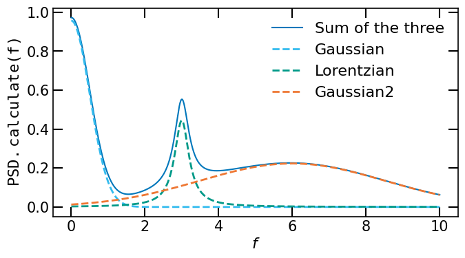
Sum of PSD functions

We can create a model which is the sum of the three components by using the + operator. The result is a new instance of the class PowerSpectralDensity. We can inspect the parameters of the model by printing the object.

Model = Lore + Gauss + Gauss2
print(Model)

Power spectrum: lorentzian + gaussian + gaussian
Number of parameters: 9
============================================================================
CID  ID   Name            Value          Status    Linked    Type            
1    1    position        3              Free      No        Hyper-parameter 
1    2    amplitude       1              Free      No        Hyper-parameter 
1    3    halfwidth       1.5            Free      No        Hyper-parameter 
2    4    position        0              Free      No        Hyper-parameter 
2    5    amplitude       1.2            Free      No        Hyper-parameter 
2    6    sigma           0.5            Free      No        Hyper-parameter 
3    7    position        6              Free      No        Hyper-parameter 
3    8    amplitude       1.4            Free      No        Hyper-parameter 
3    9    sigma           2.5            Free      No        Hyper-parameter 

Number of free parameters : 9

Because several parameters have identical names it is necessary to use the indices of the parameters to access them. CID gives the component index and ID gives the parameter index in the whole model.

print(Model.parameters[5])

2    5    amplitude       1.2            Free      No        Hyper-parameter 

Show code cell source Hide code cell source

t = jnp.linspace(0, 10, 1000)

fig, ax = plt.subplots(1, 1, figsize=(7, 4))

ax.plot(t, Model.calculate(t), label="Sum of the three")
ax.plot(t, Gauss.calculate(t), label="Gaussian", lw=2,ls="--")
ax.plot(t, Lore.calculate(t), label="Lorentzian", lw=2,ls="--")
ax.plot(t, Gauss2.calculate(t), label="Gaussian2", lw=2,ls="--")
ax.set_xlabel(r'$f$')
ax.set_ylabel(r'$\tt{PSD.calculate}(f)$')
ax.legend()
fig.tight_layout()

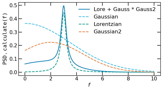
Product of PSD functions

We can create a model which is a product of PSD functions by using the * operator. The result is a new instance of the class PowerSpectralDensity. We show an example with the product of the two first components plus the third component.

Lore = Lorentzian([3,1, 1.5])
Gauss = Gaussian([0,3.2, 3.5])
Gauss2 = Gaussian([2,1.4, 2.5])

Model = Lore + Gauss * Gauss2
print(Model)

Power spectrum: lorentzian + gaussian * gaussian
Number of parameters: 9
============================================================================
CID  ID   Name            Value          Status    Linked    Type            
1    1    position        3              Free      No        Hyper-parameter 
1    2    amplitude       1              Free      No        Hyper-parameter 
1    3    halfwidth       1.5            Free      No        Hyper-parameter 
2    4    position        0              Free      No        Hyper-parameter 
2    5    amplitude       3.2            Free      No        Hyper-parameter 
2    6    sigma           3.5            Free      No        Hyper-parameter 
3    7    position        2              Free      No        Hyper-parameter 
3    8    amplitude       1.4            Free      No        Hyper-parameter 
3    9    sigma           2.5            Free      No        Hyper-parameter 

Number of free parameters : 9

Show code cell source Hide code cell source

t = jnp.linspace(0, 10, 1000)

fig, ax = plt.subplots(1, 1, figsize=(7, 4))

ax.plot(t, Model.calculate(t), label="Lore + Gauss * Gauss2", lw=2)
ax.plot(t, Gauss.calculate(t), label="Gaussian", lw=2,ls="--")
ax.plot(t, Lore.calculate(t), label="Lorentzian", lw=2,ls="--")
ax.plot(t, Gauss2.calculate(t), label="Gaussian2", lw=2,ls="--")
ax.set_xlabel(r'$f$')
ax.set_ylabel(r'$\tt{PSD.calculate}(f)$')
ax.legend()
fig.tight_layout()

Conversion to an autocovariance function

To use PSD models which have no analytical expression for the autocovariance function we have to compute the Fourier Transform of the PSD. This is done using the class PSDToACV. The class takes as input a PowerSpectralDensity object and computes the Fourier Transform of the PSD. The class has a method calculate which takes as input a list of floats representing the time lags at which the autocovariance function is evaluated. The method returns a list of floats representing the values of the autocovariance function at the given time lags.

We first define a PSD model, here a Lorentzian. We then create an instance of the class PSDToACV, four other values are necessary to do so. The total duration of the time series \(T\), \(\Delta T\) the minimal time step between two consecutive points in the time series, \(S_\mathrm{low}\) and \(S_\mathrm{high}\) two factors to extend the grid of frequencies used to compute the Fourier Transform.

The extended grid of frequencies is then given by \(f_0 = f_\mathrm{min}/S_\mathrm{low} = \Delta f\) to \(f_N = f_\mathrm{max}S_\mathrm{high}=N \Delta f\), where \(f_\mathrm{min}=1/T\) and \(f_\mathrm{max}=1/2\Delta T\). More details about these two factors can be found in the Notebook on the FFT.

System Message: WARNING/2 ([thick] \draw (0,2pt) -- + (0,-2pt) node[below=1mm] {0}; \draw (.5,2pt) -- + (0,-2pt) node[below=1mm] {$f_0$}; \draw (3.5,5pt) -- + (0,-5pt) node[below=1mm] {$f_\mathrm{min}$}; \draw (10.,5pt) -- + (0,-5pt) node[below=1mm] {$f_\mathrm{max}$}; \draw (14,5pt) -- + (0,-5pt) node[below=1mm] {$f_\mathrm{N}$}; \draw[thick] (0,0) -- node[below=7mm] {Frequency $f$} + (15,0); \foreach \x in {0,0.5,...,14.} \draw (\x cm,3pt) -- (\x cm,-3pt) node[anchor=north] {};)

!pdflatex command cannot be run

from pioran import PSDToACV

Lore = Lorentzian([0, 1, .5])
P2A = PSDToACV(PSD=Lore, S_low=10, S_high=10, T=100, dt=1, method="FFT")

We can evaluate the autocovariance of the time series at given time lags by calling the method calculate of the PSDToACV object. The method calculate takes as input a list of floats representing the time lags at which the autocovariance function is evaluated. The method returns a list of floats representing the values of the autocovariance function at the given time lags.

f = P2A.frequencies
t = jnp.linspace(0, 100, 1000)
acv = P2A.calculate(t)

We show the original PSD and the autocovariance function computed from the PSD.

Show code cell source Hide code cell source

fig, ax = plt.subplots(2, 1, figsize=(7, 7))

ax[0].loglog(f, Lore.calculate(f), label="Lorentzian")
ax[0].set_xlabel(r'$f$')
ax[0].set_ylabel(r'$\tt{PSD.calculate}(f)$')

ax[1].plot(t, acv, label="ACV")
ax[1].set_xlabel(r'$\tau$')
ax[1].set_ylabel(r'$\tt{ACV.calculate}(\tau)$')

fig.align_ylabels()
fig.tight_layout()

Writing a new model

Here we show how to write a PSD new model, which can be used like any models we have shown above.

Creating the class and the constructor

We write a new class MyPSD, which inherits from PowerSpectralDensity. It is important to specify the attributes parameters and expression at the class level since PowerSpectralDensity inherits from Module. parameters is an object of the class ParametersModel which is a container for the parameters of the model. The constructor __init__ must be defined as in the example and the names of the parameters are given in the param_names list.

The calculate method

The calculate method must be defined and it must return the PSD function evaluated at the frequencies f. When writing the expression of the PSD function, the values of parameters of the model can be accessed using the attribute self.parameters['name'].value where name is the name of the parameter.

import jax.numpy as jnp
from pioran import PowerSpectralDensity
from pioran.parameters import ParametersModel


class MyPSD(PowerSpectralDensity):
    parameters: ParametersModel
    expression = 'my_psd'
    
    def __init__(self, parameters_values, free_parameters=[True, True,True]):
        """Constructor of the power spectrum inherited 
        from the PowerSpectralDensity class.
        """
        assert len(parameters_values) == 3, 'The number of parameters must be 3'
        # initialise the parameters and check
        PowerSpectralDensity.__init__(self, param_values=parameters_values, param_names=['amplitude', 'freq','power'], free_parameters=free_parameters)
    
    def calculate(self,f):
        """Calculate the power spectrum at the given frequencies."""
        return self.parameters['amplitude'].value  /  ( 1+f/self.parameters['freq'].value)**self.parameters['power'].value

We can use the newly defined model as any other models we have shown above:

P = MyPSD([1., 0.5,3.4])
frequencies = jnp.linspace(0, 5, 1000)
PSD = P.calculate(frequencies)

Show code cell source Hide code cell source

fig, ax = plt.subplots(1,1,figsize=(7,4))
ax.plot(frequencies, PSD)
ax.set_xlabel(r'$f$')
ax.set_ylabel(r'$\tt{PSD.calculate}(f)$')
ax.loglog()
fig.tight_layout()